Periodic Sampling

A sequence of samples, x[n] is obtained from a continuous time signal \(x_c(t)\) according to the relation

\[ x[n] = x_c(nT),\quad –\infty<n<\infty \]

T is Sampling period, \(x_c(t)\) is the continuous time signal, \(x[n]\) is the discrete time signal.

Sampling frequency is \(f_s = \frac{1}{T}\).

In frequency domain, the samples frequency is \(\Omega_s = \frac{2\pi}{T}\).

The sampling processes can be represented as

\[\displaystyle{x_s(t)=x_c(t)\underbrace{\sum_{n=-\infty}^{\infty}\delta(t-nT)}_{sampling\ function\ s(t)=Ш_T}}\]

\[\displaystyle{x_s(t)=\sum_{n=-\infty}^{\infty}x_c(nT)\delta(t-nT)}\]

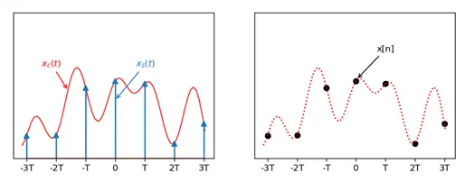
\(x_s(t)\) is a continuous time function with impulses at the sampling points and values of 0 except at the sampling points, while x[n] is a discrete time series.

Frequency Domain Representation of Sampling

Symbol	FT	DTFT	Info
\(x_c(t)\)	\(X_c(j\Omega)\)	-	Continuous time signal
\(x[n]\)	-	\(X(e^{j\omega})\)	Discrete time signal
\(x_s(t)\)	\(X(j\Omega)\)	-	Continuous time signal with impulses at sampling points
\(s(t)\)	\(S(j\Omega)\)	-	Sampling function
\(\Omega_N\)	-	-	Nyquist frequency, bandwidth of the signal
\(\Omega_s\)	-	-	Sampling frequency
T	-	-	Sampling period
\(h_r(t)\)	\(H_r(e^{j\Omega})\)	-	Reconstruction filter (continuous time)
\(h[n]\)	-	\(H(e^{j\omega})\)	impulse response (discrete time)
\(h_c(t)\)	\(H_c(e^{j\Omega})\)	-	impulse response (continuous time)

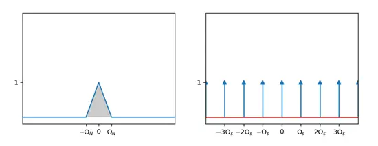
\[s(t)=\sum_{n=-\infty}^{\infty}\delta(t-nT)\]

Then we do the Fourier transform of \(s(t)\)

\[S(j\Omega)=\frac{2\pi}{T}\sum_{k=-\infty}^{\infty}\delta(\Omega-k\Omega_s)\]

\[x_s(t)=x_c(t)s(t)=x_c(t)\sum_{n=-\infty}^{\infty}\delta(t-nT)\]

Then we do the Fourier transform of \(x_s(t)\)

\[X_s(j\Omega)=\frac{1}{2\pi}X_c(j\Omega)*S(j\Omega)=\frac{1}{T}\sum_{k=-\infty}^{\infty}X_c(j(\Omega-k\Omega_s))\]

Since:

\[\begin{align*} \mathcal{F}(f\cdot g) &= \frac{1}{2\pi}F*G & \quad\mathcal{F}^{-1}(F*G) &= 2\pi f\cdot g\\ \mathcal{F}(f*g) &= F\cdot G & \quad\mathcal{F}^{-1}(F\cdot G) &= f*g \end{align*}\]

So, the simpleing result has a shifting property, \(X_s(j\Omega)\) is equivalent to the superposition of an infinite number of shifted \(\frac{1}{T}X_c(j\Omega)\).

This superposition can be categorized in two ways

Non-aliased

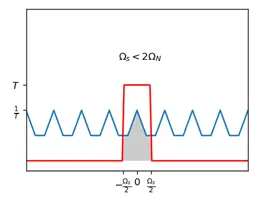
If the frequency(\(\Omega_N\)) of the Fourier transform of the continuous time signal \(X_c(j\Omega)\) is less than \(\frac{\Omega_s}{2}=\frac{\pi}{T}\), then the spectrum of \(X_s(j\Omega)\) will not overlap.

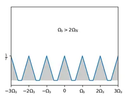
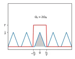
For a non-aliased spectrum, we can easily use a T-weighted (multiplied by T) low-pass filter to obtain the original spectrum, i.e., the original signal can be restored from this spectrum. ## Aliasing

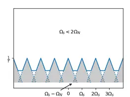
For an aliased spectrum, the original spectrum is not obtained by using a low-pass filter, and the original signal cannot be obtained.

Conclusion

Nyquist-Shannon Sampling Theorem:

Sampling a signal with a band limit of \(\Omega_N\) requires a sampling frequency of \(\Omega_s>=2\Omega_N\) to avoid aliasing.

Nyquist frequency : \(\Omega_N\) Nyquist rate : \(2\Omega_N\)

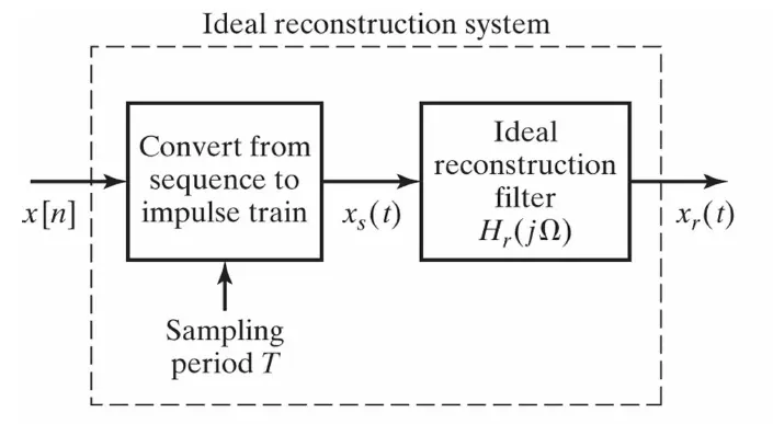
Reconstruction of Bandlimited Signal from its Samples

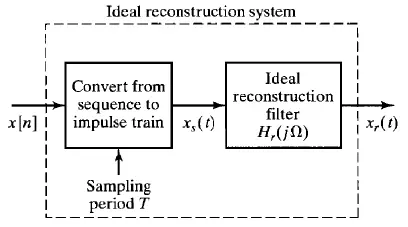
Given, x[n] and T, the impulse train is obtained as

\[x_s(t)=x_c(t)s(t)=x_c(t)\sum_{n=-\infty}^{\infty}\delta(t-nT)\]

Then

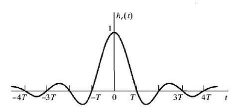
\[\begin{align*} x_r(t) &= \mathcal{F}^{-1}(X_s(j\Omega)H_r(j\Omega)) \qquad H_r(j\Omega)=\left\{\begin{matrix} T, & |\Omega|\leqslant \Omega_s/2=\frac{\pi}{T}\\ 0, & else \end{matrix}\right. \\ &= x_s(t)*h_r(t)\qquad fourier\ convolution\ theorem\\ &= \left\{ \sum_{n=-\infty}^{\infty}x[n]\delta(t-nT)\right \}*\left\{ \frac{sin(\pi t/T)}{\pi t/T} \right\}\\ &= \sum_{n=-\infty}^{\infty}x[n]\left\{\delta(t-nT) * \frac{sin(\pi t/T)}{\pi t/T} \right\}\qquad x[n]\ is\ sample\ value,constant \\ &= \sum_{n=-\infty}^{\infty}x[n]\frac{sin[\pi (t-nT)/T]}{\pi (t-nT)/T} \qquad \delta\ shift\ property \end{align*}\]

The relationship between continuous-time and discrete-time signals

C/D

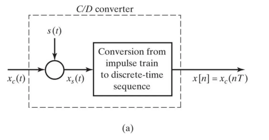
Since:

\[X_s(j\Omega)=\frac{1}{2\pi}X_c(j\Omega)*S(j\Omega)=\frac{1}{T}\sum_{k=-\infty}^{\infty}X_c(j(\Omega-k\Omega_s))\]

We can get: \[ \begin{align*} X(e^{j\omega})|_{\omega=\Omega T} &= X(e^{j\Omega T})\\ &= X(j\Omega) \\ &= \frac{1}{T}\sum_{k=-\infty}^{\infty}X_c\left( j\left( \Omega-k\Omega_s \right) \right) \\ &= \frac{1}{T}\sum_{k=-\infty}^{\infty}X_c\left[ j\left(\frac{\omega}{T}-\frac{2\pi k}{T} \right )\right ] \qquad \left\{\begin{matrix}\Omega &= &\frac{\omega}{T}\\ \Omega_s &= &\frac{2\pi}{T} \end{matrix} \right.\\ \end{align*} \]

\[\begin{align*} X(e^{j\omega}) &= \frac{1}{T}\sum_{k=-\infty}^{\infty}X_c\left[ j\left(\Omega-\frac{2\pi k}{T} \right ) \right ]\\ &= \frac{1}{T}\sum_{k=-\infty}^{\infty}X_c\left[ j\left(\frac{\omega}{T}-\frac{2\pi k}{T} \right )\right ] \qquad \omega=\Omega T \end{align*}\]

D/C

Discrete time processing of continuous time signals

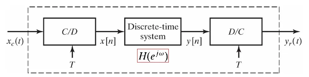
We can get:

\[\begin{align*} Y_r(j\Omega) &= H_r(j\Omega)Y(e^{j\omega}) \qquad lowpass\ filter\ H_r(j\Omega)\ for\ restruction\\ &= H_r(j\Omega)H(e^{j\omega})X(e^{j\omega})\qquad LTI\ system\ frequency\ response\ H(e^{j\omega})\\ &= H_r(j\Omega)H(e^{j\Omega T})\frac{1}{T}\sum_{k=-\infty}^{\infty}X_c\left[j\left(\Omega-\frac{2\pi k}{T} \right )\right ] \\ &=\left\{ \begin{matrix} H(e^{j\Omega T})X_c(j\Omega), & |\Omega|<\pi/T\\ 0,& |\Omega|\geqslant \pi/T\end{matrix}\right. \qquad because\ H_r(j\Omega) = \left\{\begin{matrix}T, & |\Omega|<\pi/T\\ 0, & |\Omega|\geqslant \pi/T \end{matrix}\right.\\ &= H_{eff}(j\Omega)X_c(j\Omega) \qquad H_{eff}(j\Omega) = \left\{ \begin{matrix} H(e^{j\Omega T}), & |\Omega|<\pi/T\\ 0,& |\Omega|\geqslant \pi/T\end{matrix}\right. \end{align*}\]

The CT is bandlimited \(X_c(j\Omega)=0\) for \(|\Omega|>\pi/T\)
The reconstruction filter is an ideal LPF with gain T
The sampling rate is above Nyquist rate
The processing system is an LTI system

We have:

\[\begin{align*} H_{eff}(j\Omega) &= \left\{ \begin{matrix} H(e^{j\Omega T}), & |\Omega|<\pi/T\\ 0,& |\Omega|\geqslant \pi/T\end{matrix}\right.\\ &= \left\{ \begin{matrix} \displaystyle{\frac{1}{T}\sum_{k=-\infty}^{\infty}H_{c}\left[j\left( \Omega-\frac{2\pi k}{T} \right)\right]}, & |\Omega|<\pi/T\\ 0,& |\Omega|\geqslant \pi/T\end{matrix}\right.\qquad assume\ h[n]=h_c(nT)\\ &= \left\{ \begin{matrix} \frac{H_c(j\Omega)}{T}, & |\Omega|<\pi/T\\ 0,& |\Omega|\geqslant \pi/T\end{matrix}\right.\\ \end{align*}\]

Continuous-time Processing of Discrete-time Signals

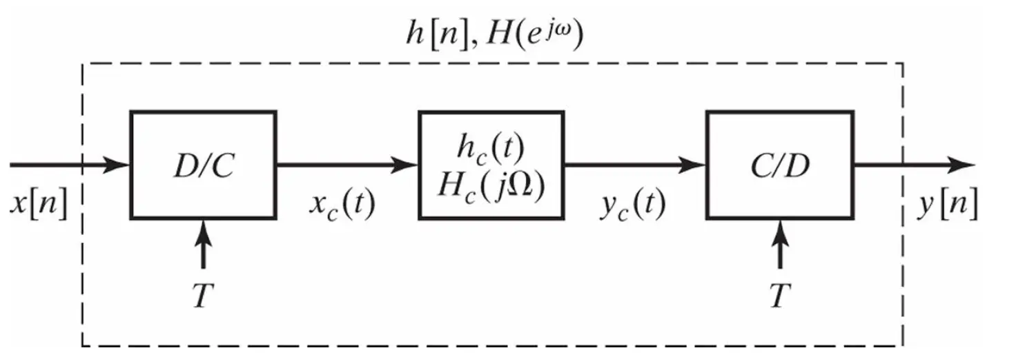
Assume that the system as well as the input signal satisfy the Nyquist sampling theorem

\[x_c(t) = \displaystyle{ \sum_{n=-\infty}^{\infty}x[n]\frac{sin[\pi(t-nT)/T]}{\pi(t-nT)/T} }\] \[y_c(t) = \displaystyle{ \sum_{n=-\infty}^{\infty}y[n]\frac{sin[\pi(t-nT)/T]}{\pi(t-nT)/T} }\]

And \(x[n] = x_c(nT),y[n] = y_c(nT)\)

\[X_c(j\Omega) = TX(e^{j\Omega T}),\qquad |\Omega|<\pi/T\]

\[Y_c(j\Omega) = H_c(j\Omega)X_c(j\Omega)\]

\[Y(e^{j\omega}) = \frac{1}{T}Y_c\left( j\frac{\omega}{T} \right),\qquad |\omega|<\pi\]

Then we can get:

\[H(e^{j\omega}) = H_c(j\frac{\omega}{T}),\qquad |\omega|<\pi\]

\[H(e^{j\Omega T}) = H_c(j\Omega),\qquad |\Omega|<\pi/T\]

Downsampling

The process of reducing the sampling rate is known as desampling

Reducing the sampling rate by an integer multiple (with a multiplicity of M) should be done by directly extracting a value every M samples from the source sample sequence

\[x_d[n] = x[nM] = x_c(nMT)\]

This extraction method is called a sample rate compressor, or compressor for short. It can be seen that the resulting new sequence is part of the original continuous signal and that the sampling period of the new sequence is Td=MT. For this new sequence, we can discuss it in two cases:

Td satisfies the Nyquist sampling theorem, i.e., the new sequence can be reduced to the original continuous signal by a low-pass filter
Td does not satisfy the Nyquist sampling theorem, i.e., the new sequence is aliased and cannot be reduced to the original continuous signal

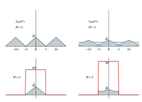
If the sequence still satisfies the Nyquist sampling theorem after employing a compressor with a compression rate of M, we can proceed directly to use xd[n] = x[Mn] to obtain a desampled sequence.

The sampling period is fixed to MT, and if a sampled signal has a sampling period of MT, then the condition that it will not be aliased after sampling is that the signal has an as-of frequency of \(\frac{\pi}{MT}\), and thus the as-of frequency of the low-pass filtering is \(\frac{\pi}{MT}\).