
Discrete-time Signal Processing (1)
Discrete-Time Signals
Define
A discrete-time signal is a sequence of numbers that are defined at discrete points in time. It is often represented as a function of an integer variable, such as \(x[n]\) or \(x(n)\), where \(n\) is the time index.
\[x={x[n]},n \in Z\]
This sequence can be sampled from a continuous-time signal \(x(t)\)
\[x[n] = x_a(nT), ,n \in Z\]
where T is the sampling period and its \(\frac{1}{T}\) is the sampling frequency.
Basic sequences
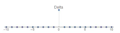
Unit sample
\[\delta[n]=\left\{\begin{matrix} 1, & n=0\\ 0, & n\neq 0 \end{matrix}\right.\]
Any sequence can be expressed as
\[x[n] = \displaystyle{ \sum_{k=-\infty}^{\infty}x[k]\delta[n-k] }\]
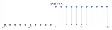
Unit step
\[u[n]=\left\{\begin{matrix} 1, & n\geq 0\\ 0, & n< 0 \end{matrix}\right.\]
It also can be expressed as
\[u[n] = \displaystyle{ \sum_{k=-\infty}^{n}\delta[k] }\]
\[u[n] = \displaystyle{ \sum_{k=0}^{\infty}\delta[n-k] }\]
\[\delta[n] = u[n] - u[n-1]\] ### Exponential
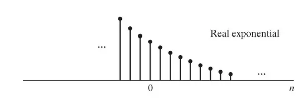
\[x[n] = Aa^n u[n]\]
If A,α are both complex numbers
\[\left\{\begin{matrix} A& = & |A|(cos\phi+jsin\phi)&=&|A|e^{j\phi} \\ \alpha & = & |\alpha|(cos\omega_0+jsin\omega_0) &=&|\alpha|e^{j\omega_0} \end{matrix}\right.\]
Then
\[\begin{align*} x[n] &= A\alpha^n\\ &= |A|e^{j\phi}|\alpha|^ne^{j\omega_0n}\\ &= |A||\alpha|^ne^{j(\omega_0n+\phi)}\\ &= |A||\alpha|^ncos(\omega_0n+\phi)+j|A||\alpha|^nsin(\omega_0n+\phi) \end{align*}\]
When \(\alpha=1\)
\[x[n] = |A|e^{j(\omega_0n+\phi)} = |A|cos(\omega_0n+\phi)+j|A|sin(\omega_0n+\phi)\] ### Sinusoid
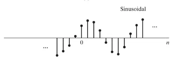
\[x[n] = A\sin(\omega_0n+\phi)\]
Difference between discrete-time sinusoidal series and continuous-time sinusoidal signals
Frequency
Assuming a frequency \((\omega_0 + 2\pi)\)
If it is a continuous time sinusoidal signal, then there are
\[f(t) = Acos((\omega_0+2\pi)t + \phi)\]
If it is a discrete-time sinusoidal signal, then there are
\[x[n] = Acos[\omega_0n+2\pi n + \phi] = Acos[\omega_0 n + \phi]\]
We can see that discrete-time sinusoidal sequences with frequency \((\omega_0 + 2\pi k)\) (where k is an arbitrary integer) are indistinguishable from each other, i.e., the frequency remains \(\omega_0\)
Period
For continuous time sinusoidal signals
\[f(t) = Acos(\omega_0t+\phi)\] The period of this signal \(T=\frac{2\pi}{\omega_0}\)
For discrete-time sinusoidal signals
\[x[n] = Acos[\omega_0n+\phi]\]
In the discrete time case, a periodic sequence should satisfy
\[x[n] = x[n+N]\]
The period N in Equation must be an integer. If this condition is used to test the periodicity of a discrete-time sinusoidal sequence, we have
\[Acos(\omega_0n+\phi) = Acos(\omega_0n+\omega_0N+\phi)\]
\[\omega_0N = 2\pi k\]
Where k is an integer. It can be seen that the value of the period N is not necessarily equal to \(\frac{2\pi}{\omega_0}\), this is because N must be an integer.
Discrete-time systems
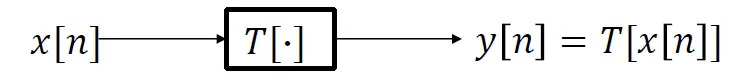
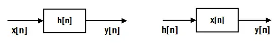
Mathematically defined as transformation that maps input sequence x[n] into an output y[n]
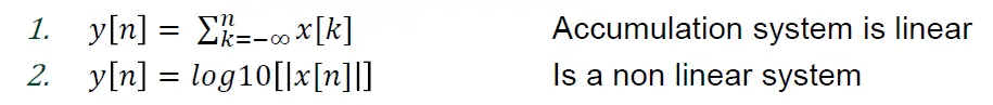
Memoryless System
If the output y[n] at every value of n depends only on the input x[n] at the same value of n.
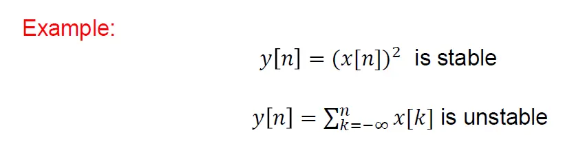
Exp. \[y[n] = (x[n])^2 , for\space each\space n\]
Linear Systems
Defined by the principle of superposition for its input and output.
It satisfies the following two conditions:
\[\begin{align*} &T\{x_1[n]+x_2[n]\} &=& T\{x_1[n]\}+T\{x_2[n]\} &=& y_1[n]+y_2[n]\\ &T\{ax[n]\}&=&aT\{x[n]\}&=&ay[n] \end{align*}\]
Where a is an arbitrary constant. The combination of
these two properties is known as the principle of superposition and is
written as
\[T\{ax_1[n]+bx_2[n]\} = aT\{x_1[n]\}+bT\{x_2[n]\}\]
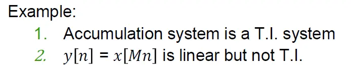
Example:
Time-Invariant Systems
A system for which a time shift or delay of the input sequence causes a corresponding shift in the output sequence. \[T\{x[n-n_0]\} = y[n-n_0]\]
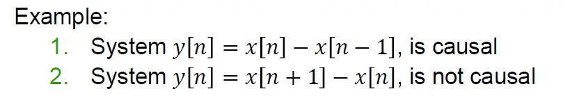
Causal Systems
When the output at sample n, i.e. y[n], only depends on the present and/or past values of input x[n]. The value of the output sequence at n = n0 depends only on the value of the input sequence at n <= n0
Stability
(in BIBO sense) A system where the response of finite inputs do not diverge.
\[|x[n]|\leqslant B_x < \infty,\ for\ each\ n\] \[|y[n]|\leqslant B_y < \infty,\ for\ each\ n\]
LTI Systems
These systems are both Linear and Time Invariant.
They have significant applications in DT signal processing.
There is a very convenient representation form for these systems, using convolutional sum.
\[y[n] = x[n]*h[n] = \sum_{k=-\infty}^{\infty}x[k]h[n-k]\]
Where * denotes convolution operation.
Where h[n] is called the impulse response of the
system.
Important Formula
\[\sum_{k=N1}^{N2}a^k = \frac{a^{N_1} - a^{N_2+1}}{1-a}\]
Properties of LTI Systems
Commutative property:
\[\begin{align*} y[n] &=x[n]*h[n] \\ &=\sum_{m=-\infty}^{\infty}x[n-m]h[m] \\ &=\sum_{p=-\infty}^{\infty}x[p]h[n-p] \quad letting\ p=n-m \\ &=\sum_{p=-\infty}^{\infty}h[n-p]x[p] \\ &=h[n]*x[n] \end{align*}\]
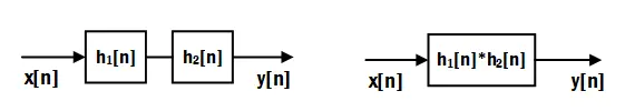
Associative property:
\[\begin{align*} y[n] &=(x[n]*h_1[n])*h_2[n] \\ &=z[n]*h_2[n] \\ &=\sum_{m=-\infty}^{\infty}z[n-m]h_2[m] \\ &=\sum_{p=-\infty}^{\infty}z[p]h_2[n-p] \quad letting\ p=n-m\\ &=\sum_{p=-\infty}^{\infty}\left ( \sum_{i=-\infty}^{\infty}x[p-i]h_1[i] \right )h_2[n-p] \\ &=\sum_{p=-\infty}^{\infty}\left ( \sum_{q=-\infty}^{\infty}x[q]h_1[p-q] \right )h_2[n-p] \quad letting\ q=p-i\\ &=\sum_{q=-\infty}^{\infty}x[q]\left ( \sum_{p=-\infty}^{\infty}h_1[p-q]h_2[n-p] \right ) \\ &=\sum_{q=-\infty}^{\infty}x[q]\left ( \sum_{m=-\infty}^{\infty}h_1[n-q-m]h_2[m] \right ) \\ &=\sum_{k=-\infty}^{\infty}x[n-k]\left ( \sum_{m=-\infty}^{\infty}h_1[k-m]h_2[m] \right ) \quad letting\ k=n-q \\ &=x[n]*(h_1[n]*h_2[n]) \end{align*}\]
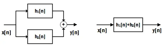
Distributive property:
\[\begin{align*} y[n] &=x[n]*h[n] \\ &=x[n]*(h_1[n]+h_2[n]) \\ &=\sum_{m=-\infty}^{\infty}x[n-m](h_1[m]+h_2[m]) \\ &=\sum_{m=-\infty}^{\infty}x[n-m]h_1[m]+\sum_{m=-\infty}^{\infty}x[n-m]h_2[m] \\ &=x[n]*h_1[n]+x[n]*h_2[n] \end{align*}\]
Time shifting property:
If \(𝑦[𝑛] = 𝑥[𝑛] ∗ ℎ[𝑛]\) , then \(𝑥[𝑛 − 𝑛1] ∗ ℎ [𝑛 − 𝑛2] = 𝑦 [𝑛 − 𝑛1 − 𝑛2]\)
Causallity:
An LTI system is causal if and only if \(ℎ[𝑛] = 0\) for \(𝑛 < 0\) , then \(𝑦[𝑛] = 0\) for \(𝑛 < 0\)
Finite
If 𝑥[𝑛] and ℎ[𝑛] are of finite duration, then 𝑦[𝑛] is of finite duration.
In particular, if 𝑥[𝑛] is of length 𝑁1, and ℎ[𝑛] is of length 𝑁2, then 𝑦[𝑛] is of length 𝑁1 +𝑁2 −1.
Stability:
An LTI system is BIBO stable if and only if \[\sum_{k=-\infin}^{\infin}|ℎ[k]| < \infin\]
EXAMPLE
Delay system
\[y[n] = x[n-n_d]\]
\[h[n] = \delta[n-n_d]\]
Moving averag
\[y[n] = \frac{1}{M_1+M_2+1}\displaystyle{ \sum_{k=-M_1}^{M_2}x[n-k] }\]
\[\begin{align*} h[n] &=\frac{1}{M_1+M_2+1}\sum_{k=-M_1}^{M_2}\delta[n-k] \\ &=\left \{\begin{matrix} \frac{1}{M_1+M_2+1}, & -M_1\leqslant n\leqslant M_2 \\ 0, & \ else \end{matrix}\right.\\ &=\frac{1}{M_1+M_2+1}(u[n+M_1]-u[n-M_2-1]) \\ &=\frac{1}{M_1+M_2+1}(\delta[n+M_1]-\delta[n-M_2-1])*u[n] \end{align*}\]
Accumulator
\[y[n] = \displaystyle{ \sum_{k=-\infty}^{n}x[k] }\]
\[\begin{align*} h[n] &= \sum_{k=-\infty}^{n}\delta[k]\\ &=\sum_{k=-\infty}^{0}\delta[n+k] \\ &= \left\{\begin{matrix} 1 &,n\geqslant 0 \\ 0 &,n<0 \end{matrix}\right. \\ &=u[n] \end{align*}\]
Forward difference
\[y[n] = x[n+1]-x[n]\]
\[h[n] = \delta[n+1]-\delta[n]\]
Backward difference
\[y[n] = x[n]-x[n-1]\]
\[h[n] = \delta[n]-\delta[n-1]\]
Linear Constant-Coefficient Difference Equations
They are an important class of LTI systems where the input x[n] and the output y[n] satisfy an Nth order linear constant coefficient difference equation as follows:
\[\displaystyle{ \sum_{k=0}^{N}a_k y[n-k]=\sum_{m=0}^{M}b_m x[n-m] }\]
When we solve the difference equation, we will assume \(y_h[n] = Az^n\)
Then we can get
\[\displaystyle{ \sum_{k=0}^{N}a_k z^{-k} } = 0\] \[y_h[n] = \displaystyle{ \sum_{m=1}^{N}A_m z_m^n }\]
initial-rest condition
\[if\ x[n]=0,\ n<n_0 \quad then \ y[n]=0,\ n<n_0 \]
Frequency domain representation of signals and systems
For an LTI system, if the input is \(x[n] = e^{j\omega n},-\infty<n<\infty\) then the output is
\[\begin{align*} y[n] &= \sum_{k=-\infty}^{\infty}h[k]x[n-k] \\ &=\sum_{k=-\infty}^{\infty}h[k]e^{j\omega(n-k)}\\ &=\sum_{k=-\infty}^{\infty}h[k]e^{-j\omega k}e^{j\omega n} \end{align*}\]
\[H(e^{j\omega}) = \displaystyle{ \sum_{k=-\infty}^{\infty}h[k]e^{-j\omega k} }\]
It can be observed that eigenvalues \(H(e^{j\omega})\) are a function ω of frequency dependent, so eigenvalues \(H(e^{j\omega})\) are also known as the frequency response of the system. Generally, \(H(e^{j\omega})\) it is a complex number and can be divided into real and imaginary representations
\[H(e^{j\omega}) = H_R(e^{j\omega}) + jH_I(e^{j\omega})\]
\[H(e^{j\omega}) = |H(e^{j\omega})|e^{j\angle H(e^{j\omega)}}\]
And the Frequency response has periodicity.
\[\begin{align*} H(e^{j(\omega+2\pi)}) &= \sum_{n=-\infty}^{\infty}h[n]e^{-j(\omega+2\pi)n} \\ &= \sum_{n=-\infty}^{\infty}h[n](e^{-j\omega n}e^{-j2\pi n})\\ &= \sum_{n=-\infty}^{\infty}h[n]e^{-j\omega n}\\ &= H(e^{j\omega}) \end{align*}\]
If
\[x[n] = Acos (\omega_0 + \phi) = \frac{A}{2}e^{j\phi}e^{j\omega_0 n} + \frac{A}{2}e^{-j\phi}e^{-j\omega_0 n}\]
Then
\[\begin{align*} y[n] &= \frac{A}{2}\{H(e^{j\omega_0})e^{j\theta}e^{j\omega_0 n}+H(e^{-j\omega_0})e^{-j\theta}e^{-j\omega_0 n} \} \\ &= \frac{A}{2}\{[H_R(e^{j \omega_0})+jH_I(e^{j\omega_0})]e^{j\theta}e^{j\omega_0 n}+[H_R(e^{j \omega_0})-jH_I(e^{j\omega_0})]e^{-j\theta}e^{-j\omega_0 n} \} \\ &\qquad h[n]\ is\ real\Rightarrow H(e^{-j\omega_0})=H^{*}(e^{j\omega_0})\\ &= \frac{A}{2}\{ H_R(e^{j\omega_0})(e^{j\theta}e^{j\omega_0 n}+e^{-j\theta}e^{-j\omega_0 n})+jH_I(e^{j\omega_0})(e^{j\theta}e^{j\omega_0 n}-e^{-j\theta}e^{-j\omega_0 n}) \} \\ &= \frac{A}{2} \{ 2H_R(e^{j\omega_0})cos(\omega_0 n + \theta) - 2H_I(e^{j\omega_0})sin(\omega_0 n + \theta) \} \\ &= A \{ H_R(e^{j\omega_0})cos(\omega_0 n + \theta) - H_I(e^{j\omega_0})sin(\omega_0 n + \theta) \} \\ &= A\{ |H(e^{j\omega_0})|cos(\phi)cos(\omega_0 n +\theta)-|H(e^{j\omega_0})|sin(\phi)sin(\omega_0 n +\theta)\} \quad letting\ \phi=\angle H(e^{j\omega_0})\\ &= A |H(e^{j\omega_0})| cos(\omega_0 n +\theta+\phi) \end{align*}\]
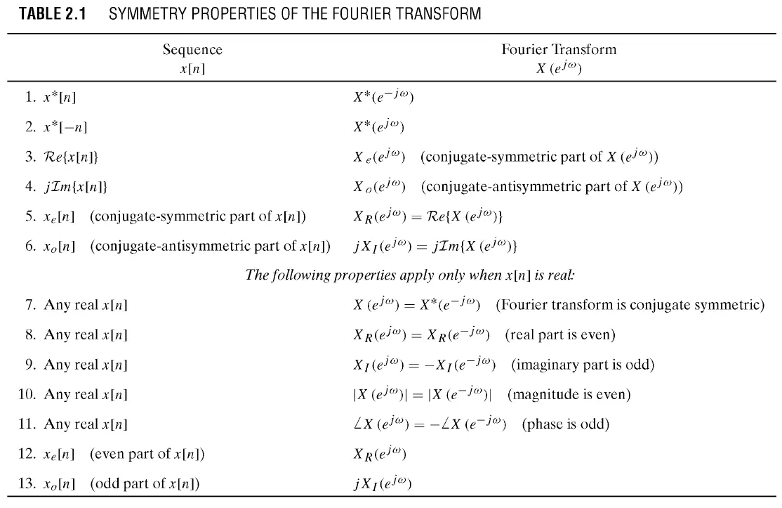
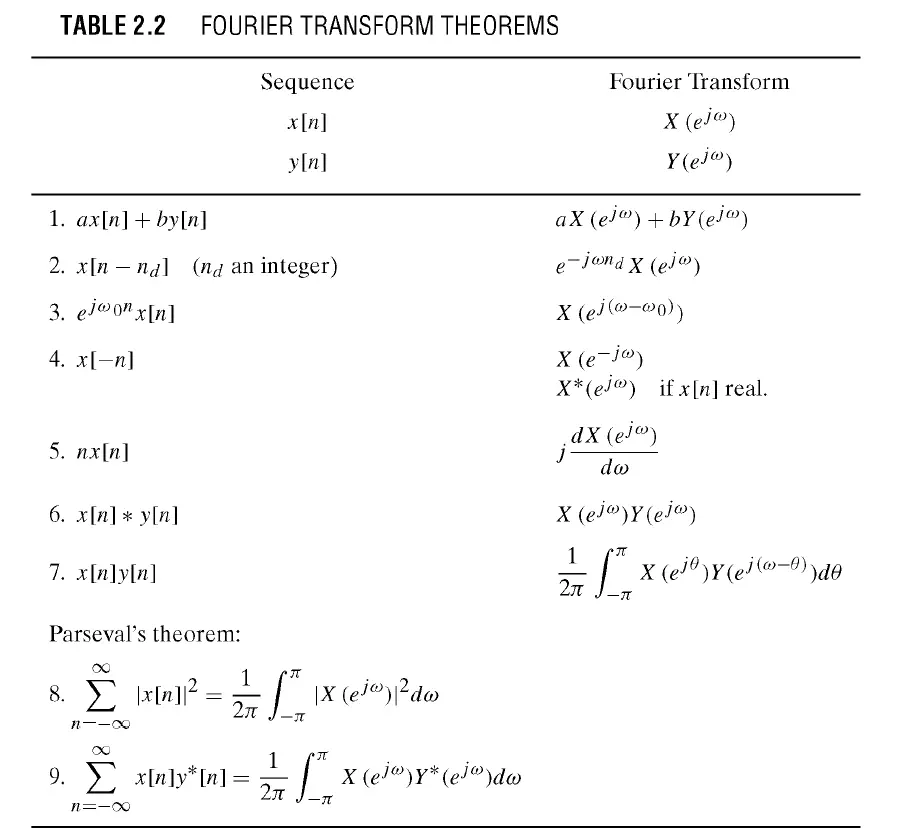
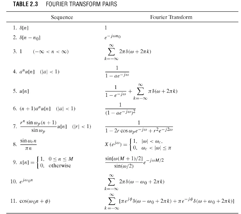
Discrete-Time Fourier Transform
\[{X(e^{j\omega}) = \displaystyle{ \sum_{n=-\infty}^{\infty}x[n]e^{-j\omega n} }}\]
\[{\displaystyle{x[n] = \frac{1}{2\pi}\int_{-\pi}^{\pi}X(e^{j\omega})e^{j\omega n}d\omega }}\]
\[x[n] = x_e[n]+x_o[n]\]
\[\left\{\begin{matrix} x_e[n] &=&\frac{1}{2}(x[n]+x^*[-n]) &=&x_e^*[-n] \\ x_o[n] &=&\frac{1}{2}(x[n]-x^*[-n]) &=&-x_o^*[-n] \end{matrix}\right.\]
\[X(e^{j\omega}) = X_e(e^{j\omega})+X_o(e^{j\omega})\]
\[\left\{\begin{matrix} X_e(e^{j\omega}) &=&\frac{1}{2}[X(e^{j\omega})+X^*(e^{j\omega})] &=&X_e^*(e^{j\omega}) \\ X_o(e^{j\omega}) &=&\frac{1}{2}[X(e^{j\omega})-X^*(e^{j\omega})] &=&-X_o^*(e^{j\omega}) \end{matrix}\right.\]
 wechat
 alipay