Machine learning--数学相关(1)
Vectors(向量)
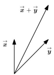
Geometric vectors
Polynomials(多项式)
2个polynomicals 可以加到一起成为另外一个polynomical
Audio signals(音频信号)
Audio signals are represented as a series of numbers.可以 add signals together, 然后他们的和就是另外一个audio signal.
Linear Equations(线性方程)
\[\begin{array}{c}
a_{11} x_{1}+\cdots+a_{1 n} x_{n}=b_{1} \\
\vdots \\
a_{m 1} x_{1}+\cdots+a_{m n} x_{n}=b_{m}
\end{array}\] 可以转换成
\[\left[\begin{array}{c}
a_{11} \\
\vdots \\
a_{m 1}
\end{array}\right] x_{1}+\left[\begin{array}{c}
a_{12} \\
\vdots \\
a_{m 2}
\end{array}\right] x_{2}+\cdots+\left[\begin{array}{c}
a_{1 n} \\
\vdots \\
a_{m n}
\end{array}\right] x_{n}=\left[\begin{array}{c}
b_{1} \\
\vdots \\
b_{m}
\end{array}\right]\] 写成Matrice(矩阵)形式 \[\left[\begin{array}{ccc}
a_{11} & \cdots & a_{1 n} \\
\vdots & & \vdots \\
a_{m 1} & \cdots & a_{m n}
\end{array}\right]\left[\begin{array}{c}
x_{1} \\
\vdots \\
x_{n}
\end{array}\right]=\left[\begin{array}{c}
b_{1} \\
\vdots \\
b_{m}
\end{array}\right]\]
Matrices(矩阵)
\[\boldsymbol{A}=\left[\begin{array}{cccc} a_{11} & a_{12} & \cdots & a_{1 n} \\ a_{21} & a_{22} & \cdots & a_{2 n} \\ \vdots & \vdots & & \vdots \\ a_{m 1} & a_{m 2} & \cdots & a_{m n} \end{array}\right], \quad a_{i j} \in \mathbb{R}\] (m,n)matrix A consist of m rows and n columns
Matrix Addition and Multiplicationc
Sum
The sum of two matrices A,B is defined as the element-wise(元素层面) sum \[\boldsymbol{A}+\boldsymbol{B}:=\left[\begin{array}{ccc} a_{11}+b_{11} & \cdots & a_{1 n}+b_{1 n} \\ \vdots & & \vdots \\ a_{m 1}+b_{m 1} & \cdots & a_{m n}+b_{m n} \end{array}\right] \in \mathbb{R}^{m \times n}\]
multiplication
For matrices A(mn), B(nk), the elements \(c_{i,j}\) of the product C=AB(m*k) are
computed as \[c_{i j}=\sum_{l=1}^{n} a_{i l}
b_{l j}\] 用\(A\cdot B\)来denote
multiplication. 其中 Matrices can only be multiplied if their
"neighboring" dimensions match, like this \[\underbrace{\boldsymbol{A}}_{n \times k}
\underbrace{\boldsymbol{B}}_{k \times m}=\underbrace{\boldsymbol{C}}_{n
\times m}\] 具体计算过程可以参考下面公式
For \(\boldsymbol{A}=\left[\begin{array}{lll}1
& 2 & 3 \\ 3 & 2 & 1\end{array}\right] \in \mathbb{R}^{2
\times 3}, \boldsymbol{B}=\left[\begin{array}{cc}0 & 2 \\ 1 & -1
\\ 0 & 1\end{array}\right] \in \mathbb{R}^{3 \times 2}\) , we
obtain
\[\begin{aligned} \boldsymbol{A} \boldsymbol{B} &=\left[\begin{array}{lll} 1 & 2 & 3 \\ 3 & 2 & 1 \end{array}\right]\left[\begin{array}{cc} 0 & 2 \\ 1 & -1 \\ 0 & 1 \end{array}\right]=\left[\begin{array}{cc} 2 & 3 \\ 2 & 5 \end{array}\right] \in \mathbb{R}^{2 \times 2} \\ \boldsymbol{B} \boldsymbol{A} &=\left[\begin{array}{cc} 0 & 2 \\ 1 & -1 \\ 0 & 1 \end{array}\right]\left[\begin{array}{ccc} 1 & 2 & 3 \\ 3 & 2 & 1 \end{array}\right]=\left[\begin{array}{ccc} 6 & 4 & 2 \\ -2 & 0 & 2 \\ 3 & 2 & 1 \end{array}\right] \in \mathbb{R}^{3 \times 3} \end{aligned} \]
Identity matrix(单位矩阵)
\[\boldsymbol{I}_{n}:=\left[\begin{array}{cccccc} 1 & 0 & \cdots & 0 & \cdots & 0 \\ 0 & 1 & \cdots & 0 & \cdots & 0 \\ \vdots & \vdots & \ddots & \vdots & \ddots & \vdots \\ 0 & 0 & \cdots & 1 & \cdots & 0 \\ \vdots & \vdots & \ddots & \vdots & \ddots & \vdots \\ 0 & 0 & \cdots & 0 & \cdots & 1 \end{array}\right] \in \mathbb{R}^{n \times n}\]
Notice
满足一些formula
\[(AB)C=A(BC)\] \[(A+B)C=AC+BC\] \[A(C+D)=AC+AD\] \[I_m A=A I_n=A\]
Inverse and Transpose
Inverse
Consider a square matrix \(\boldsymbol{A} \in \mathbb{R}^{n \times n}\). Let matrix \(\boldsymbol{B} \in \mathbb{R}^{n \times n}\) have the property that \(\boldsymbol{A} \boldsymbol{B}=\boldsymbol{I}_{n}=\boldsymbol{B} \boldsymbol{A}\). \(\boldsymbol{B}\) is called the inverse of \(\boldsymbol{A}\) and denoted by \(\boldsymbol{A}^{-1}\).
Not every matrix A possesses an inverse \(A^{-1}\). If this inverse does exist, A is called regular/ invertible/ nonsingular, otherwise singular/ noninvertible. When the matrix inverse exist, it is unique.
Transpose
For \(\boldsymbol{A} \in \mathbb{R}^{m \times n}\) the matrix \(\boldsymbol{B} \in \mathbb{R}^{n \times m}\) with \(b_{i j}=a_{j i}\) is called the transpose of \(\boldsymbol{A}\). We write \(\boldsymbol{B}=\boldsymbol{A}^{\top}\).
Notice
满足以下一些formula \[ \begin{aligned} \boldsymbol{A} \boldsymbol{A}^{-1} &=\boldsymbol{I}=\boldsymbol{A}^{-1} \boldsymbol{A} \\ (\boldsymbol{A} \boldsymbol{B})^{-1} &=\boldsymbol{B}^{-1} \boldsymbol{A}^{-1} \\ (\boldsymbol{A}+\boldsymbol{B})^{-1} & \neq \boldsymbol{A}^{-1}+\boldsymbol{B}^{-1} \\ \left(\boldsymbol{A}^{\top}\right)^{\top} &=\boldsymbol{A} \\ (\boldsymbol{A}+\boldsymbol{B})^{\top} &=\boldsymbol{A}^{\top}+\boldsymbol{B}^{\top} \\ (\boldsymbol{A} \boldsymbol{B})^{\top} &=\boldsymbol{B}^{\top} \boldsymbol{A}^{\top} \end{aligned} \]
Multiplication by a Scalar(标量)
Let \(\boldsymbol{A} \in \mathbb{R}^{m \times n}\) and \(\lambda \in \mathbb{R}\). Then \(\lambda \boldsymbol{A}=\boldsymbol{K}, K_{i j}=\lambda a_{i j}\). Practically, \(\lambda\) scales each element of \(\boldsymbol{A}\). For \(\lambda, \psi \in \mathbb{R}\), the following holds:
Associativity: \[ (\lambda \psi) \boldsymbol{C}=\lambda(\psi \boldsymbol{C}), \quad \boldsymbol{C} \in \mathbb{R}^{m \times n} \] \[\lambda(\boldsymbol{B C})=(\lambda \boldsymbol{B}) \boldsymbol{C}=\boldsymbol{B}(\lambda \boldsymbol{C})=(\boldsymbol{B} \boldsymbol{C}) \lambda, \quad \boldsymbol{B} \in \mathbb{R}^{m \times n}, \boldsymbol{C} \in \mathbb{R}^{n \times k}\] Note that this allows us to move scalar values around. \[(\lambda \boldsymbol{C})^{\top}=\boldsymbol{C}^{\top} \lambda^{\top}=\boldsymbol{C}^{\top} \lambda=\lambda \boldsymbol{C}^{\top}$ since $\lambda=\lambda^{\top}$ for all $\lambda \in \mathbb{R}\] Distributivity: \[ \begin{array}{ll} (\lambda+\psi) \boldsymbol{C}=\lambda \boldsymbol{C}+\psi \boldsymbol{C}, & \boldsymbol{C} \in \mathbb{R}^{m \times n} \\ \lambda(\boldsymbol{B}+\boldsymbol{C})=\lambda \boldsymbol{B}+\lambda \boldsymbol{C}, & \boldsymbol{B}, \boldsymbol{C} \in \mathbb{R}^{m \times n} \end{array} \] If we define \[ \boldsymbol{C}:=\left[\begin{array}{ll} 1 & 2 \\ 3 & 4 \end{array}\right] \] then for any \(\lambda, \psi \in \mathbb{R}\) we obtain \[ \begin{aligned} (\lambda+\psi) \boldsymbol{C} &=\left[\begin{array}{cc} (\lambda+\psi) 1 & (\lambda+\psi) 2 \\ (\lambda+\psi) 3 & (\lambda+\psi) 4 \end{array}\right]=\left[\begin{array}{cc} \lambda+\psi & 2 \lambda+2 \psi \\ 3 \lambda+3 \psi & 4 \lambda+4 \psi \end{array}\right] \\ &=\left[\begin{array}{cc} \lambda & 2 \lambda \\ 3 \lambda & 4 \lambda \end{array}\right]+\left[\begin{array}{cc} \psi & 2 \psi \\ 3 \psi & 4 \psi \end{array}\right]=\lambda \boldsymbol{C}+\psi \boldsymbol{C} \end{aligned} \]
Compact representations of Systems of linear equations
For example:
\[ \begin{aligned} &2 x_{1}+3 x_{2}+5 x_{3}=1 \\ &4 x_{1}-2 x_{2}-7 x_{3}=8 \\ &9 x_{1}+5 x_{2}-3 x_{3}=2 \end{aligned} \] and use the rules for matrix multiplication, we can write this equation system in a more compact form as \[ \left[\begin{array}{ccc} 2 & 3 & 5 \\ 4 & -2 & -7 \\ 9 & 5 & -3 \end{array}\right]\left[\begin{array}{l} x_{1} \\ x_{2} \\ x_{3} \end{array}\right]=\left[\begin{array}{l} 1 \\ 8 \\ 2 \end{array}\right] \]
Solving systems of linear equations
Particular and General Solution(特解和通解)
Example:
\[ \left[\begin{array}{cccc} 1 & 0 & 8 & -4 \\ 0 & 1 & 2 & 12 \end{array}\right]\left[\begin{array}{l} x_{1} \\ x_{2} \\ x_{3} \\ x_{4} \end{array}\right]=\left[\begin{array}{c} 42 \\ 8 \end{array}\right] \]
The system has two equations and four unknows. In general we would expect infinitely many solutions. This system of equations is in a particularly easy form, where the first two columns consist of a 1 and a 0. Remember that we want to find scalars x1,...x4, such that \(\sum_{i=1}^{4} x_{i} \boldsymbol{c}_{i}=\boldsymbol{b}\), where we define ci to be the \(i^th\) column of the matrix and b the right-hand-side of above formula. A solution to the problem in this example can be found immediately by taking 42 times the first column and 8 times the second column so that. \[ \boldsymbol{b}=\left[\begin{array}{c} 42 \\ 8 \end{array}\right]=42\left[\begin{array}{l} 1 \\ 0 \end{array}\right]+8\left[\begin{array}{l} 0 \\ 1 \end{array}\right] \] Therefore, a solution is \([42,8,0,0]^{\top}\). This solution is called a particular solution or special solution. However, this is not the only solution of this system of linear equations. To capture all the other solutions, we need to be creative in generating 0 in a non-trivial way using the columns of the matrix: Adding 0 to our special solution does not change the special solution. To do so, we express the third column using the first two columns (which are of this very simple form) \[ \left[\begin{array}{l} 8 \\ 2 \end{array}\right]=8\left[\begin{array}{l} 1 \\ 0 \end{array}\right]+2\left[\begin{array}{l} 0 \\ 1 \end{array}\right] \] So that \(\mathbf{0}=8 \boldsymbol{c}_{1}+2 \boldsymbol{c}_{2}-1 \boldsymbol{c}_{3}+0 \boldsymbol{c}_{4}\) and \(\left(x_{1}, x_{2}, x_{3}, x_{4}\right)=(8,2,-1,0)\). In fact, any scaling of this solution by \(\lambda_{1} \in \mathbb{R}\) produces the \(\mathbf{0}\) vector, i.e., \[ \left[\begin{array}{cccc} 1 & 0 & 8 & -4 \\ 0 & 1 & 2 & 12 \end{array}\right]\left(\lambda_{1}\left[\begin{array}{c} 8 \\ 2 \\ -1 \\ 0 \end{array}\right]\right)=\lambda_{1}\left(8 \boldsymbol{c}_{1}+2 \boldsymbol{c}_{2}-\boldsymbol{c}_{3}\right)=\mathbf{0} \]
Following the same line of reasoning, we express the fourth column of the matrix in this example using the first two columns and generate another set of non-trivial versions of 0 as \[ \left[\begin{array}{cccc} 1 & 0 & 8 & -4 \\ 0 & 1 & 2 & 12 \end{array}\right]\left(\lambda_{2}\left[\begin{array}{c} -4 \\ 12 \\ 0 \\ -1 \end{array}\right]\right)=\lambda_{2}\left(-4 \boldsymbol{c}_{1}+12 \boldsymbol{c}_{2}-\boldsymbol{c}_{4}\right)=\mathbf{0} \]
for any \(\lambda_{2} \in \mathbb{R}\). Putting everything together, we obtain all solutions of the equation system in the example, which is called the general solution, as the set (以上的步骤是分辨设每个未知数为0,求出满足方程时别的未知数的大小,最终得到通解) \[ \left\{\boldsymbol{x} \in \mathbb{R}^{4}: \boldsymbol{x}=\left[\begin{array}{c} 42 \\ 8 \\ 0 \\ 0 \end{array}\right]+\lambda_{1}\left[\begin{array}{c} 8 \\ 2 \\ -1 \\ 0 \end{array}\right]+\lambda_{2}\left[\begin{array}{c} -4 \\ 12 \\ 0 \\ -1 \end{array}\right], \lambda_{1}, \lambda_{2} \in \mathbb{R}\right\} \]
Elementary Transformations(初等变换)
Can easyly understand by looking at the example below.
Example
\[ \begin{array}{rlllrlrlrlr} -2 x_{1} & + & 4 x_{2} & - & 2 x_{3} & - & x_{4}&+&4 x_{5} & = & -3 \\ 4 x_{1} & - & 8 x_{2} & + & 3 x_{3} & - & 3 x_{4} & + & x_{5} & = & 2 \\ x_{1} & - & 2 x_{2} & + & x_{3} & - & x_{4} & + & x_{5} & = & 0 \\ x_{1} & - & 2 x_{2} & & & - & 3 x_{4}&+&4 x_{5} & = & a \end{array} \]
We start by convertiong this system of equations into the compact
matrix notation Ax=b. We no longer mention the variables x explicitly
and build the augmented matrix ( in the form [A|b]) \[
\left[\begin{array}{rrrrr|r}
-2 & 4 & -2 & -1 & 4 & -3 \\
4 & -8 & 3 & -3 & 1 & 2 \\
1 & -2 & 1 & -1 & 1 & 0 \\
1 & -2 & 0 & -3 & 4 & a
\end{array}\right]
\] where we used the verical line to separate the left-hand side
from the right-hand side in the equation.
Swapping Rows 1 and 3 leads to
\[
\left[\begin{array}{rrrrr|r}
1 & -2 & 1 & -1 & 1 & 0 \\
4 & -8 & 3 & -3 & 1 & 2 \\
-2 & 4 & -2 & -1 & 4 & -3 \\
1 & -2 & 0 & -3 & 4 & a
\end{array}\right] \begin{array}{r}
-4 R_{1} \\
+2 R_{1} \\
-R_{1}
\end{array}
\] When we now apply the indicated transformations,we obtain
\[
\begin{array}{l}
\left[\begin{array}{rrrrr|r}
1 & -2 & 1 & -1 & 1 & 0 \\
0 & 0 & -1 & 1 & -3 & 2 \\
0 & 0 & 0 & -3 & 6 & -3 \\
0 & 0 & -1 & -2 & 3 & a
\end{array}\right]\begin{array}{r}
\\
\\
\\
-R_{2}-R_{3}
\end{array}
\\
\leadsto\left[\begin{array}{rrrrr|r}
1 & -2 & 1 & -1 & 1 & 0 \\
0 & 0 & -1 & 1 & -3 & 2 \\
0 & 0 & 0 & -3 & 6 & -3 \\
0 & 0 & 0 & 0 & 0 & a+1
\end{array}\right]\begin{array}{r}
\\
\cdot\left(-1\right)\\
\cdot\left(-\frac{1}{3}\right)\\
\end{array}\\
\rightsquigarrow\left[\begin{array}{rrrrr|r}
1 & -2 & 1 & -1 & 1 & 0 \\
0 & 0 & 1 & -1 & 3 & -2 \\
0 & 0 & 0 & 1 & -2 & 1 \\
0 & 0 & 0 & 0 & 0 & a+1
\end{array}\right]
\end{array}
\] Then we get the new equation \[
\begin{array}{rlllrlrlrlr}
x_{1}&-&2 x_{2}&+&x_{3}&-&x_{4}&+&x_{5}
& = & 0 \\
&&&& x_{3}&-&x_{4}&+&3 x_{5} & =
& -2 \\
& &&&&& x_{4}&-&2 x_{5} & = & 1
\\
& & &&&&& & 0 & = & a+1
\end{array}
\] Only for a =-1 this system can be solved. A particular
solution is \[
\left[\begin{array}{l}
x_{1} \\
x_{2} \\
x_{3} \\
x_{4} \\
x_{5}
\end{array}\right]=\left[\begin{array}{c}
2 \\
0 \\
-1 \\
1 \\
0
\end{array}\right]
\] The general solution, which captures the set of all possible
solutions, is \[
\left\{\boldsymbol{x} \in \mathbb{R}^{5}:
\boldsymbol{x}=\left[\begin{array}{c}
2 \\
0 \\
-1 \\
1 \\
0
\end{array}\right]+\lambda_{1}\left[\begin{array}{l}
2 \\
1 \\
0 \\
0 \\
0
\end{array}\right]+\lambda_{2}\left[\begin{array}{c}
2 \\
0 \\
-1 \\
2 \\
1
\end{array}\right], \quad \lambda_{1}, \lambda_{2} \in
\mathbb{R}\right\}
\]
Calculation the inverse
the method calls Gaussian Elimination
Example: To determine the inverse of \[ \boldsymbol{A}=\left[\begin{array}{llll} 1 & 0 & 2 & 0 \\ 1 & 1 & 0 & 0 \\ 1 & 2 & 0 & 1 \\ 1 & 1 & 1 & 1 \end{array}\right] \] we write down the augmented matrix \[ \left[\begin{array}{llll|llll} 1 & 0 & 2 & 0 & 1 & 0 & 0 & 0 \\ 1 & 1 & 0 & 0 & 0 & 1 & 0 & 0 \\ 1 & 2 & 0 & 1 & 0 & 0 & 1 & 0 \\ 1 & 1 & 1 & 1 & 0 & 0 & 0 & 1 \end{array}\right] \] and use Gaussian elimination to bring it into reduced row-echelon form \[ \left[\begin{array}{cccc|cccc} 1 & 0 & 0 & 0 & -1 & 2 & -2 & 2 \\ 0 & 1 & 0 & 0 & 1 & -1 & 2 & -2 \\ 0 & 0 & 1 & 0 & 1 & -1 & 1 & -1 \\ 0 & 0 & 0 & 1 & -1 & 0 & -1 & 2 \end{array}\right], \] such that the ddesired inverse is given as its right-hand side: \[ \boldsymbol{A}^{-1}=\left[\begin{array}{cccc} -1 & 2 & -2 & 2 \\ 1 & -1 & 2 & -2 \\ 1 & -1 & 1 & -1 \\ -1 & 0 & -1 & 2 \end{array}\right] \] 将原矩阵和一个单位矩阵拼接在一起形成一个增广矩阵(augmented matrix) 对这个矩阵进行初等变换( Elementary Transformations)将左边变换为单位矩阵,则右边的矩阵就为原矩阵的逆矩阵
Algorithms for solving a system of linear equations
As for ordinary square matrix and invertible. We can use this formula to solve the question.
\[\boldsymbol{A} \boldsymbol{x}=\boldsymbol{b}\] \[\boldsymbol{x}=\boldsymbol{A}^{-1} \boldsymbol{b}\]
For other matrix in different structure, we use the formula below to solve the question. \[ \boldsymbol{A x}=\boldsymbol{b} \Longleftrightarrow \boldsymbol{A}^{\top} \boldsymbol{A} \boldsymbol{x}=\boldsymbol{A}^{\top} \boldsymbol{b} \Longleftrightarrow \boldsymbol{x}=\left(\boldsymbol{A}^{\top} \boldsymbol{A}\right)^{-1} \boldsymbol{A}^{\top} \boldsymbol{b} \]
 wechat
 alipay