Adaptable image segmentation via simple pixel classification

Introduction

Their image segmentation method combines 3 features: 1. Do not need to employ complex features(like color, texture, edge or other spaces) to return a better segmentation accuracies. 2. It uses a simple yet flexible multiscale spproach to local pixel heighborhood delineation, which is inspired by the concept of foveation. So it leads to a linear rather than a quadratic increase in the 3. It is a readily parallelizable segmentation algorithm

Method

Training phase

Input GT images(include hue, saturation, value and intensity or HSVI format) to train.

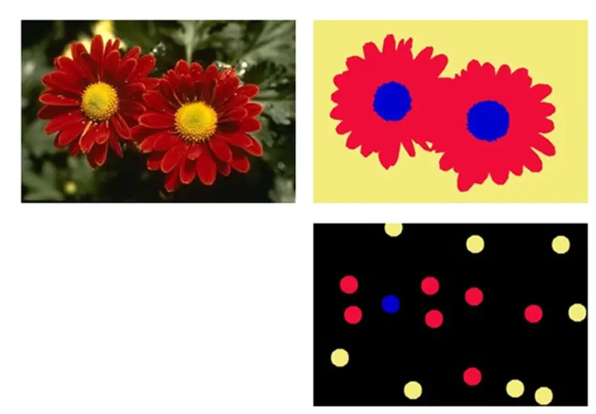training_set A set of training images.The upper right quarter and the lower right quarter of this Figure contain the full GT and partial GT images corresponding to the OI in the upper left quarter column.

This method limite the number of classes in cureent implementation to 64, including a no-class class.

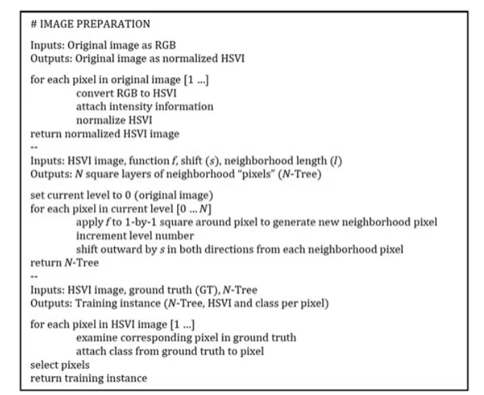
Then construct a special data structure, called N-tree. N-tree is made of N plains of "pixels". A pxel(\(P_{i,j,m-1}\))at position(i,j) within a given layer(m), excecpt for layer 0( which is given),is a selectabel function(f)(eg, Gaussian blur) of a resizabel square neighborhood(\(N_{l,s}\)) with odd-valued length \(l\) and shift \(s\) of the equivalent pixel in the preceding level (m-1)

\[P_{i,j,m}=f(N_{l,s}(P_{i,j,m-1}))\]

look at the example below. \(l=3\) and \(s=3\). Each pixel in the neighborhood N at level 1 results from the application of function \(f\) to the underlying 3*3 neighborhood of pixels at level0. At level 2, a pixel comes from function f as applied to 9 pixels from level 1. However, these 9 pixels are not adjacent but are shifted apart by 3 pixels, in both dimensions. At level 3, a pixel results from the application of function f to 9 pixels also, but these pixels are now separated by \(3^2\) pixels. Generally, shift \(s\) between pixels in the square neighborhood of a central pixel at level m is equal to \(l^{m-1}\).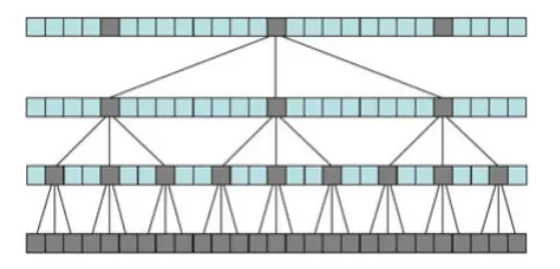

This Figure show a 2-dimensional slice of a 3*3 N-tree built using a shift value of 3, with levels 0,1,2 and 3 is showm. The lowermost layer is level 0, which is the original image

The whole process of preparing of Image can be seen from the image.

And the flow chart we can see below: 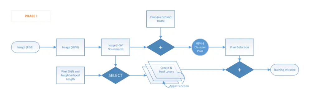phase1 Phase1 shows how to prepare the training instance.

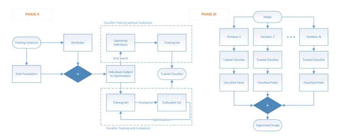phase2,3 Phase2 shows how to training classifer and Phase3 shows how to segmented images.

Experimental setup

Test measures

This research uses the flowing formula to represent the effect of each methods. The measure algorithm we can see below. \[TP\%=\frac{TP count}{TP count+FN count}*100\]

TP means true positive, FP means false positive, TN means negative and FN means false negative.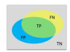

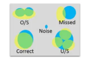This figure shows 5 different results which will be return by the classifier. Yellow regions are regions from the GT image, while blue regions come from the machine-segmented(MS)image, and gray is the background. O/S is an oversegmented region(means segmented region is larger than the actural area); U/S is an undersegmented region(means segmented region is lower than the actural area); correct is a correctly segmented region, while a missed region is not correctly segmented or O/S or U/S; Noise is an MS region with no ground truth equivalent.