Water_Extracting
In this project, I design a neural network structure to achieve the target of extracting water body from the remote sensing images. And finally it achive a better result than other previously methods.
Target
In urban features, water bodies influence the functioning of urban ecosystems in various ways, with their role in, for example, tourism, flood control and urban heat island regulation constantly influencing human life and urban economic development. There for a objective and accurate understanding of the spatial and temporal distribution characteristics of urban water resources is essential for urban planning and development. To achieve this target, designing an effective and reliable method to help human to extract this data from remote sensing images more quicklly is useful and necessary. In this situation, designing an artificial inteligent method to achieve this goal base on deep learning is suitable.
Method
Data processing
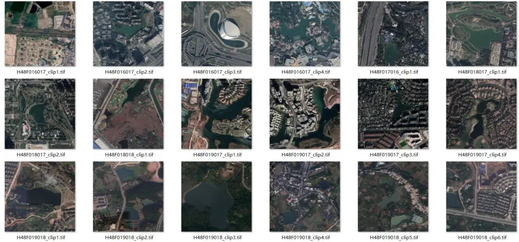
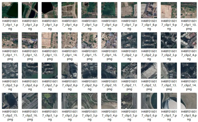
First of all, we need to get the data that is used to train the deep
learining algorithms. I choose download the remote sensing images of
Chengdu, China from the Google Earth Engine. I have acquired almost 40
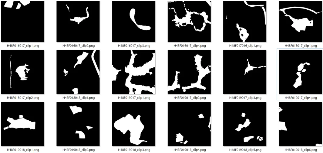
images of 4000*4000. Then I use the ArcMap to make the lable of each
image, to creat the data of training.
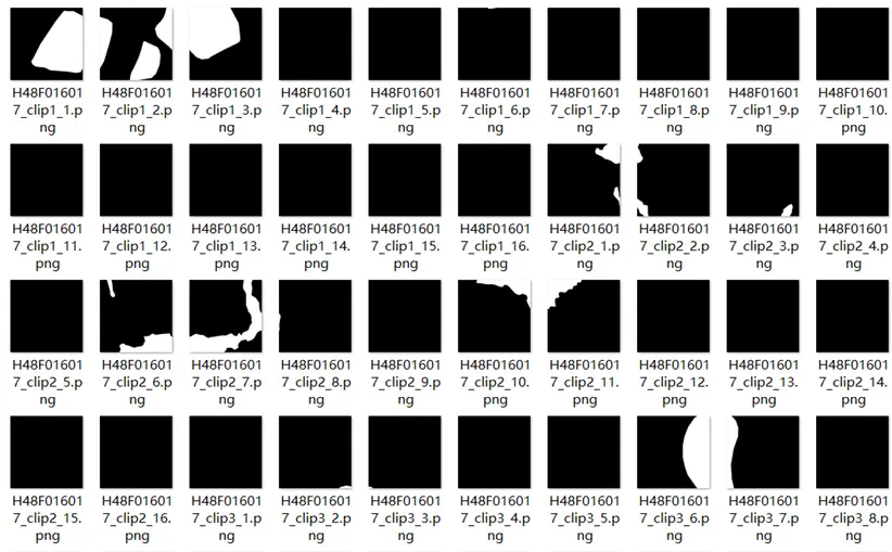
To enhance the robustness and generalisation of the network, it is
often necessary to augment the training data. In this project, the
existing dataset was randomly transformed by mirroring, vertical
transformation, cropping, random selection, fuzzy processing and noise
addition operations, eventually expanding the dataset to 10000 images of
512*512. 1
2
3
4
5
6
7
8
9
10
11
12
13
14
15
16
17def gamma_transform(img, gamma):
gamma_table = [np.power(x / 255.0, gamma) * 255.0 for x in range(256)]
gamma_table = np.round(np.array(gamma_table)).astype(np.uint8)
return cv2.LUT(img, gamma_table)
def random_gamma_transform(img, gamma_vari):
log_gamma_vari = np.log(gamma_vari)
alpha = np.random.uniform(-log_gamma_vari, log_gamma_vari)
gamma = np.exp(alpha)
return gamma_transform(img, gamma)
def rotate(xb,yb,angle,img_w,img_h):
M_rotate = cv2.getRotationMatrix2D((img_w/2, img_h/2), angle, 1)
xb = cv2.warpAffine(xb, M_rotate, (img_w, img_h))
yb = cv2.warpAffine(yb, M_rotate, (img_w, img_h))
return xb,yb
def blur(img):#加模糊
img = cv2.blur(img, (3, 3));
return img
Network structure
In this projcet, I improve the traditional Unet structure, like the
image shows below. 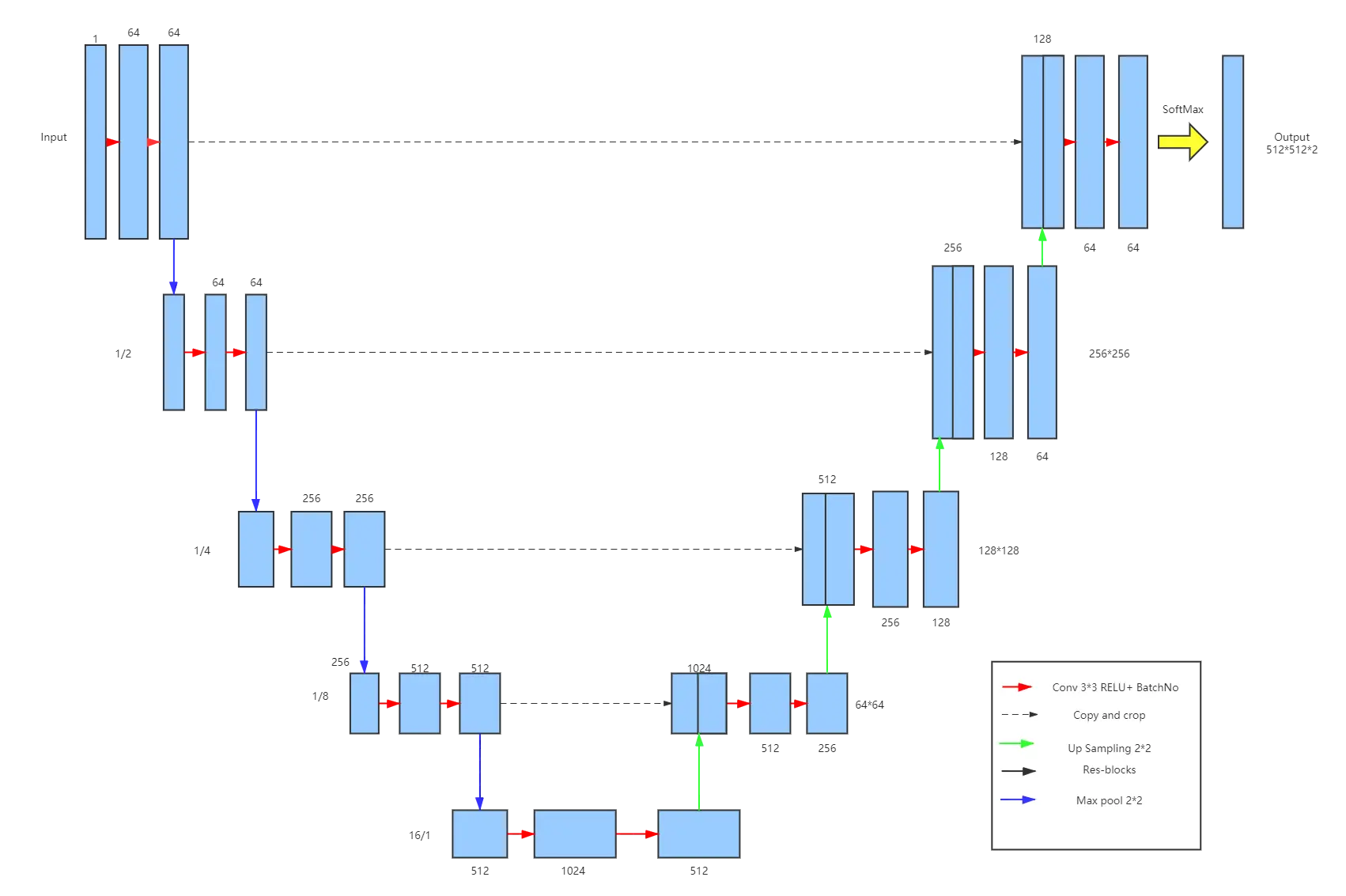 A deeper network structure is designed based on Unet,
while Dilated convolution is used to implement feature map downsampling
and feature extraction to further improve the accuracy and
generalisation of the network extraction. Meanwhile, I introduce the
Res-block that is a good solution to the problem of network degradation
that can occur when the network structure is too deep.
A deeper network structure is designed based on Unet,
while Dilated convolution is used to implement feature map downsampling
and feature extraction to further improve the accuracy and
generalisation of the network extraction. Meanwhile, I introduce the
Res-block that is a good solution to the problem of network degradation
that can occur when the network structure is too deep. 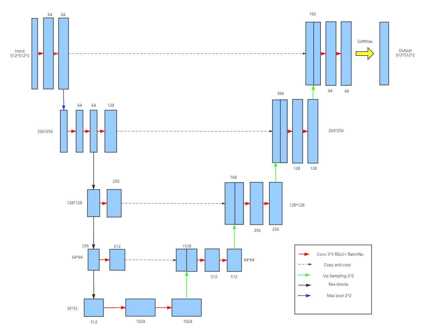
1
2
3
4
5
6
7
8
9
10
11
12
13
14
15
16
17
18
19
20
21
22
23
24
25
26
27
28
29
30
31
32
33
34
35
36
37
38
39
40
41
42
43
44
45
46
47
48
49
50
51
52
53
54
55
56
57
58
59
60
61
62
63
64
65
66
67
68
69
70
71
72
73
74
75
76
77def __init__(self, num_classes=2, in_channels=3, pretrained=False,record=False):
super(MyUnet2, self).__init__()
out_filters = [64, 128, 256, 512,1024]
resnet = models.resnet34(pretrained=True)
self.record=record
self.encoder1 = resnet.layer1
self.encodecov1=nn.Sequential(
nn.Conv2d(out_filters[0],out_filters[1], kernel_size=3, padding=1),
nn.ReLU(True),
nn.BatchNorm2d(out_filters[1]),
)
self.encoder2 = resnet.layer2
self.encodecov2=nn.Sequential(
nn.Conv2d(out_filters[1],out_filters[2], kernel_size=3, padding=1),
nn.ReLU(True),
nn.BatchNorm2d(out_filters[2]),
)
self.encoder3 = resnet.layer3
self.encodecov3=nn.Sequential(
nn.Conv2d(out_filters[2],out_filters[3], kernel_size=3, padding=1),
nn.ReLU(True),
nn.BatchNorm2d(out_filters[3]),
)
self.encoder4 = resnet.layer4
self.encodecov4=nn.Conv2d(out_filters[3],out_filters[4],kernel_size=3,padding=1)
self.Down1 = unetDown(in_channels, out_filters[0])
self.Down2 = unetDown(out_filters[0], out_filters[1])
self.Down3 = unetDown(out_filters[1], out_filters[2])
self.Down4 = unetDown2(out_filters[2], out_filters[3])
self.Down5 = unetDown3(out_filters[3], out_filters[4])
self.Up1=unetUp(out_filters[4], out_filters[3])
self.Up2=unetUp(out_filters[3], out_filters[2])
self.Up3=unetUp(out_filters[2], out_filters[1])
self.Up4=unetUp(out_filters[1], out_filters[0])
self.cov111=nn.Conv2d(out_filters[0],2,kernel_size=3,padding=1)
self.relu=nn.ReLU(True)
self.final = nn.Conv2d(2, num_classes, 1)
self.maxp=nn.MaxPool2d(kernel_size=2, stride=2)
self.finalsof=nn.Softmax(dim=-1)
def forward(self, inputs):
feate1=self.Down1(inputs)
feate11=self.maxp(feate1)
e1 = self.encoder1(feate11)#64,512,512
e11=self.encodecov1(e1)
e2 = self.encoder2(e1)#128,256,256
e21=self.encodecov2(e2)
e3 = self.encoder3(e2)#256,128,128
e31=self.encodecov3(e3)
e4 = self.encoder4(e3)#512,64,64
feate5=self.Down5(e4)
Up6=self.Up1(e31,feate5)
Up7=self.Up2(e21,Up6)
Up8=self.Up3(e11,Up7)
Up9=self.Up4(feate1,Up8)
final=self.cov111(Up9)
final=self.relu(final)
final=self.final(final)
return final
def _initialize_weights(self, *stages):
for modules in stages:
for module in modules.modules():
if isinstance(module, nn.Conv2d):
nn.init.kaiming_normal_(module.weight)
if module.bias is not None:
module.bias.data.zero_()
elif isinstance(module, nn.BatchNorm2d):
module.weight.data.fill_(1)
module.bias.data.zero_()
Dilated convolution
It refers to the injection of uncomputed voids into the standard
convolution kernel, as shown in the figure, and in this way increases
the perceptual range of the network 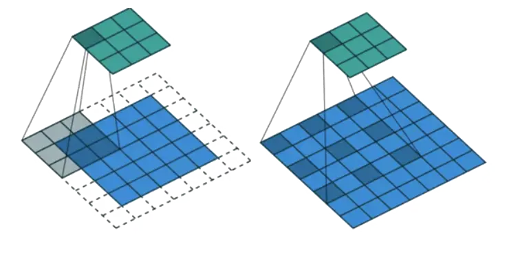
Res-Block
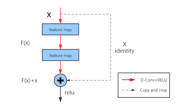 This structure does not complicate the computation
during training and no other parameters are generated to consume memory.
And it can also help to retain both low-dimensional and high-dimensional
features of the feature map.
This structure does not complicate the computation
during training and no other parameters are generated to consume memory.
And it can also help to retain both low-dimensional and high-dimensional
features of the feature map.
loss function
In this projcet, a combined loss function combining a pixel-based cross-entropy loss function and a Disce loss function is used as the overall training loss function. The combination of the two loss functions allows the simultaneous acquisition of CE-loss capable of pixel-based computation, while using Dice loss to balance the disadvantage of unreliable CE-loss performance when the ratio of water to non-water bodies in the image is out of balance.
CE-loss
The cross-entropy loss function is by far the most commonly used loss function for image semantic segmentation tasks. This method examines each pixel point individually and compares the class predictions with the one-hot encoded label. The equation implemented is as follows \[ \operatorname{loss}=\sum_{j} t_{i, j} \log \left(y_{i, j}\right)+\left(1-t_{i, j}\right) \log \left(1-y_{i, j}\right) \]
Dice loss
The formula is implemented as follows, in effect finding the overlap between the two samples \[ \operatorname{loss}=1-\frac{2|A \cap B|}{|A|+|B|} \]
Result
Accuracy Evaluation
The main accuracy evaluation methods used in this paper are F-score, kappa coefficient, and MIoU coefficient.
F-score
\[ F-\text { score }=\frac{\left(1+\beta^{2}\right) \text { precision } \times \text { recall }}{\beta^{2} \text { precision }+\text { recall }} \] \[ \begin{array}{r} \text { precision }=\frac{T P}{T P+F P} \\ \text { recall }=\frac{T P}{T P+F N} \end{array} \]
Kappa coefficient
\[ K=\frac{N \sum_{i=1}^{r} x_{i i}-\sum_{i=1}^{r}\left(x_{i+} \times x_{+i}\right)}{N^{2}-\sum_{i=1}^{r}\left(x_{i+} \times x_{+i}\right)} \]
\(\mathrm{MlOU}\) coefficient
\[ \mathrm{MlOU}=\frac{1}{k+1} \sum_{i=0}^{k} \frac{p_{i i}}{\sum_{j=0}^{k} p_{i j}+\sum_{i=0}^{k} p_{j i}-p_{i i}} \] Equal \[ \mathrm{MlOU}=\frac{1}{k+1} \sum_{i=0}^{k} \frac{T P}{F N+F P+T P} \]
Result
| Network Structure | F-SCORE | KAPPA | MIOU |
|---|---|---|---|
| DEEPLABV3+ | 0.901 | 0.812 | 93.85% |
| UNET | 0.966 | 0.899 | 96.58% |
| DLINKNET | 0.911 | 0.794 | 93.32% |
| RES-UNET | 0.939 | 0.968 | 98.85% |
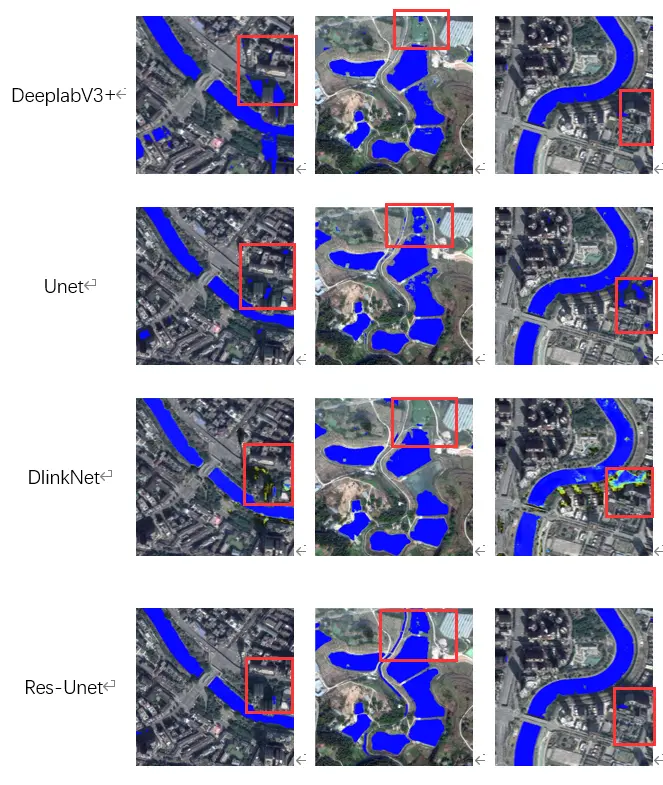 This picture shows the effect of each network structures
in extracting water bodies from remote sensing images.
This picture shows the effect of each network structures
in extracting water bodies from remote sensing images.
Through these data we can see the ResUnet structure provided in this paper had the highest MIoU at 98.85% and the highest Kappa index at 0.968. This indicates that the ResUnet model was able to extract the vast majority of the water bodies and also had the highest accuracy.
Finally
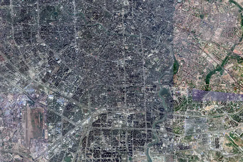 Use this algorithm to extract water body from the
93696*62464 remote sensing image of Chengdu China.
Use this algorithm to extract water body from the
93696*62464 remote sensing image of Chengdu China. 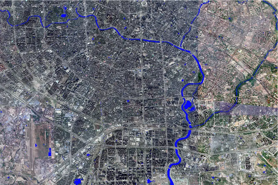 This took only about 10 minutes.
More detail about the codes of this project you can check from my GitHub.
 wechat
 alipay